Release planning is critical for Scrum teams. This post offers a practical way to assess whether a set of features can be delivered within a release. By simulating quarterly planning in Jupyter Notebook, we explore what’s possible, the likelihood of dropping features, and address the key question: can we deliver the planned portfolio with statistical confidence? Building on this foundation, the following approach details how specific simulations are used.
To build based on this foundation, the approach simulates the number of story points per feature for each release. It then estimates both the expected cost and the cost at risk, where cost at risk is defined as the maximum cost at the 95th percentile—i.e., a conservative estimate of the potential highest cost that might reasonably occur in 95 out of 100 scenarios.
Simulation Parameters
When planning a release, you can define various parameters. Most are straightforward. Sprint uncertainty is the spread of previous Sprint estimations. Higher sprint uncertainty occurs when attempting new tasks, such as a spike, when the team changes due to crises, compliance needs, restructuring, or when the team is new to the product or services. The sprint ceiling is a parameter that represents the highest level of underestimation observed in previous sprints. The cancellation threshold is a parameter that indicates that if a feature exceeds its planned duration by more than 2 sprints, there is a 60% likelihood that it will be canceled.
Parameter blockchain.yaml | Case-study value | Planning meaning |
|---|---|---|
sprint_length_weeks | 2 weeks | Defines the time box and translates Sprint demand into calendar time and delivery rhythm. |
quarterly_capacity_sprints | 6 sprints | Defines how many Sprint slots fit into the quarter; this is the parameter behind the visible 8-vs-6 overload. |
delay_model.sprint_uncertainty | 30% | Controls how wide the simulated spread around the planned Sprint count is. |
delay_model.sprint_ceiling | 2.5x | Caps extreme overruns so the simulated delay stays within a plausible range. |
cancellation.max_sprints_over_plan | > 2 sprints | Defines when the stop/continue gate becomes active for a late feature. |
cancellation.cancellation_probability | 60% | Defines how often a feature is cancelled once that gate has been crossed. |
Effort and Outcomes
Figure 1 shows what delay uncertainty does to a Sprint plan. For each feature, the simulation draws thousands of scenarios from a truncated lognormal distribution, moment-matched to the planned Sprint count. The shape mirrors what real teams experience: most scenarios finish close to plan, a smaller share runs significantly late, and a fraction is cancelled at the gate.
Effort is the number of Sprints a feature needs to finish, derived from the estimated development weeks and rounded up to whole Sprints. Two outcomes can move the result. An overrun still ships the feature, but consumes more Sprints than planned; every extra Sprint adds development cost and reduces capacity for other work. A cancellation fires once the simulated Sprint count exceeds the planned count by more than the configured threshold — the feature does not ship, business value drops to zero, and the cost accrued up to the trigger is sunk.
The right tail of the distribution carries both. That tail is where the budget surprises live.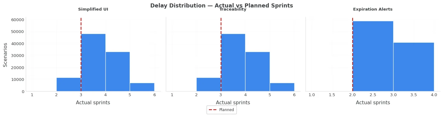
In the chart, each red dashed line indicates the planned Sprint count. The blue bars represent the frequency with which the simulation matches the plan, overruns, or is canceled at the gate. The histogram distinguishes between overruns and cancellations for each feature. In daily planning, these outcomes are often combined as “it took longer.”
Development Costs
The notebook replaces a single planned cost figure with four: Planned Cost, Expected Cost (the average including delay risk), Cost at Risk 95% (the 95th percentile), and CVaR 95% (the average cost in the worst 5% of cases). These metrics define the baseline budget, escalation threshold, and funding appetite.
Budget pressure is a metric that is the ratio:
This ratio shows, as a percentage, how much the worst-case expected cost exceeds the planned investment. Because the metric is proportional, a small feature with a tight margin can show more pressure than a large one with plenty of room.
$$ \text{Budget pressure} = \frac{\mathrm{CVaR}_{95}}{C_{\text{plan}}} - 1 $$For the case study, the simulation produces these per-feature values:
| Feature | Planned | Expected | CaR 95% | CVaR 95% | Budget pressure |
|---|---|---|---|---|---|
| H1 Simplified UI | 75,000 EUR | 104,286 EUR | 150,000 EUR | 153,302 EUR | +104.4% |
| H2 Traceability | 55,000 EUR | 76,500 EUR | 110,000 EUR | 112,437 EUR | +104.4% |
| H3 Expiration Alerts | 10,509 EUR | 17,608 EUR | 28,024 EUR | 28,272 EUR | +169.0% |
Figure 2 visualises these four cost levels per feature. For every feature, the bars rise from the Planned baseline to Expected, then to CaR 95% and CVaR 95%. Expected sits above Planned because the right-skewed delay distribution makes overruns more likely than early completion. CVaR sits slightly above CaR because the worst 5 % of scenarios continue beyond the 95th-percentile boundary.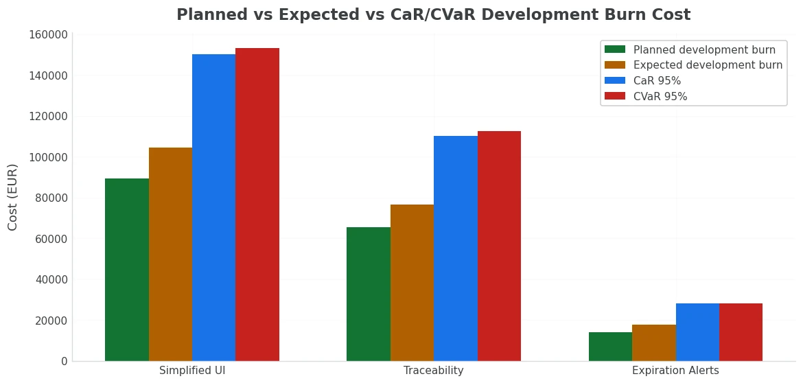
The chart shows that the cheapest feature has the highest budget pressure. Expiration Alerts (H3) is budgeted at around EUR 10k, but its worst-case cost is 169% over budget. Adding another Sprint almost doubles the planned investment. Larger features go over budget by 104%. This comparison highlights budget pressure for features of all sizes.
Summary
This is my favorite notebook in the series because it matches how teams work. It is ideal for the most common decision-making processes in agile work, such as Roadmap creation, Backlog prioritization, and Refinements.
These methods are not often used outside of financial institutions. By simulating effort, this notebook reflects what teams and stakeholders already think about: how much Sprint capacity a feature uses and what the worst-case cost could be in euros.
Rather than just providing a single planned number, the notebook lays out four different cost levels: Planned, Expected, CaR 95%, and CVaR 95%. It also includes a Budget Pressure metric that’s easy to compare. This lets you spot possible worst-case scenarios, but without making it feel like you’re predicting the future.
To see how useful it is, try using your own data—like past Sprint uncertainty, sprint ceilings, and delay boundaries from real releases.
Please remind Goodhart’s Laws:
“When a measure becomes a target, it ceases to be a good measure" — Goodhart’s Law
→ Inspect the notebook, scenario, and Product Owner case study on GitHub
Information
- Reading guide — Notebook 06: Development Cost Risk
- Executable notebook — 06: 06-blockchain-case-study-development-risk.ipynb
- Scenario inputs: blockchain.yaml
- GitHub repository: feature-hypotheses-simulation-public
- Product Owner Case Study: six-step decision walkthrough
- Background — Spike: Wikipedia
- Background — Lognormal distribution: Wikipedia
- Background — CVaR / Expected shortfall: Wikipedia
- Background — Goodhart’s Law: Wikipedia
- Related post: Feature Hypotheses Simulation
- Related post: Business Value
- Related post: Risk Resilience — the portfolio-risk companion to this post.